8 How to Write Functions
As I said a few chapters ago, R programming runs on objects. Most object types relate to the way data is stored and how it’s handled. There’s one object type, though, that’s unique compared to the others.
That would be the function object type.
R functions allow you to script out various commands to transform and analyze data. This can be as simple as taking data from a vector and outputting a data frame. Or it could be something as complicated as a machine learning algorithm!
It all depends on your own R programming goals.
8.1 Two Approaches to Using R Functions
There’s two approaches that you can take with functions:
- use an existing function
- write your own function
Both methods use the same underlying structure.
The more common functions you’ll use include those in the R base and stats packages. These automatically come with R. These functions perform common calculations needed for statistical programming, such as mean(), sum(), sd(), lm(), glm() and confint().
Other functions include those developed by other R programmers, which you can access by installing and loading other packages. (See the chapter on R packages for more details.)
8.2 Why You Should Learn to Write Your Own Functions
R is flexible enough though that you can write your own functions as well. This might sound like more trouble than it’s worth, but it’s really not. It takes a lot of time to learn other people’s functions. Not only that, you have to verify that their functions perform accurately. That’s especially true for packages developed by lesser known organizations.
Another problem is documentation. Much of the documentation for lesser known packages and their functions are poorly written. It’s easy to misunderstand their inputs and how to use them correctly. I experience this often. I’ve saved a lot of development time simply by writing my own functions.
One last benefit relates to data management. Custom functions are handy for dealing with large, unstructured data sets. You can write specific instructions that can run on a loop until you’ve cycled through the various data points. This is actually a really big deal. In a few lines of code, you can accomplish what most people would need a paid tool like Alteryx to do.
8.3 The Components of an R Function
Regardless of whether you use an existing function or write your own, both require the same components to execute: an argument and a value.
These are the technical terms for it, but it might be easier to think of an argument as the input and the value as the output.
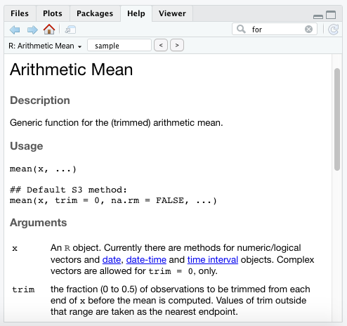
Fortunately, R documentation tells you what the required arguments are for existing functions. Simply add a question mark ? before a function and the documentation will appear in the Help tab on the bottom right pane of RStudio.
Try it yourself with these functions:
  ?mean
  ?sd
  ?cor
  ?confint
With the mean function, we see that it requires at least an x value. The Arguments section of the documentation states that x is merely a vector.
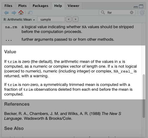
The Value section will provide details on the output for this function.
8.4 Required versus Non-Required Arguments
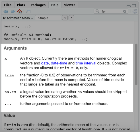
You may have noticed in the documentation for the mean() function that there were two other arguments: trim and na.rm.
You can still execute the mean() function without those arguments. The reason is that there’s a default setting already in place for them.
Whoever created this function set the default for the trim to 0 and the na.rm argument to FALSE. That way the user only has to modify those arguments if they want to.
8.5 When Order Matters for Arguments
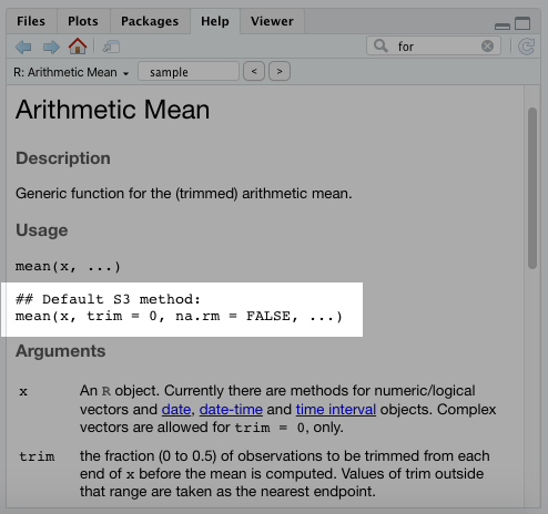
If you execute ?lm in your console, you’ll see the linear model function has argument options for formula, data, subset, weights, etc. That means we could execute the model using our Bond data as lm(gross~actor,bond). Even though we don’t specify the arguments, R will execute this function because the formula argument (gross~actor) and the data argument (bond) are placed in the correct order.
You can see this order in the documentation:
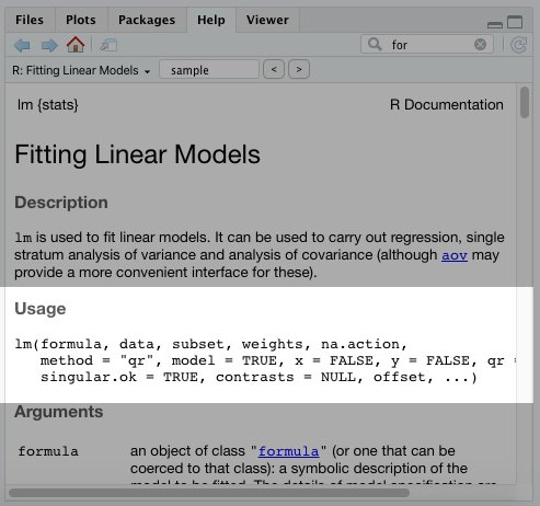
If we tried this backwards, it wouldn’t work. Executing lm(bond,gross~actor) in your console would throw up an error. However, if we specify the arguments with an equal = sign, it will execute. That would look like this: lm(data=bond,formula=gross~actor).
8.6 How to Write Your Own Functions
As you may have noticed, existing R functions require at least one argument (with the option for more) and displays at least one value as an output. If you write your own functions, they’ll need the same thing.
According to R’s own base documentation, a function is defined by an assignment, such as:
name <- function(arg_1, arg_2, …) expressionWe’re going to follow this convention and create several functions, with each one becoming more and more complex.
Our end goal will be to create a function that:
- takes a data set
- groups data based on a single categorical variable
- calculates the mean and standard deviation of a continuous variable
But first, let’s start with a simpler version of this.
For these examples, you’ll need our James Bond data set. Go ahead and re-load it with the script below:
bond <- read.csv("https://raw.githubusercontent.com/taylorrodgers/bond/main/bond.csv")Our first function will calculate standard deviation for a continuous variable.
We’ll need to provide a name for the function and any arguments to pass through. I’ll name the function sd.simple.
We also know it’ll require a data frame and a field to calculate standard deviation. I’ll call those data and field, respectively.
You can see in the script below the template for a function and the new name and arguments that I replaced it with.
  # Template
  name <- function(arg_1, arg_2, …) expression
  # New function
  sd.simple <- function(data, field) expression
Now we’ll need to add an expression. An expression is the actual script that takes your arguments and uses them to execute certain tasks.
To start the expression part of a new function, we use the {} notations:
  sd.simple <- function(data, field) {
  }
Next, we need the function to evaluate the data frame that’s placed in the data argument and select the field that’s specified. To do this, we use the same methods we used for selecting data from a data frame. (Note: when you design functions, it’s important to keep in mind the type of objects that will be entered into a function.)
If you recall, we can select a field directly from a data frame like this:
bond[,"gross"]We can use this same structure in our function. Down below, I replace “bond” and “gross” with the argument names inside the function.
  sd.simple <- function(data,field) {
    field <- data[,paste(field)]
  }
Now you probably realized that I actually replaced “gross” with paste(field). The paste() function is a useful one to remember. It comes in handy when writing your own functions. It allows you to dynamically inject an argument throughout your function’s expression.
Next, we need to write a script to calculate standard deviation. We’ll use the sample standard deviation equation, which is:
\[ \sqrt{\frac{\sum{(X_i-\bar{X})^2}}{n-1}} \]
And we’ll plug that into our function:
  sd.simple <- function(data,field) {
    field <- data[,paste(field)]
    sqrt(sum((field - mean(field))^2) / (length(field) - 1))
  }
And walla! We created our first function! To run this function, we simply add two arguments (data set and variable).
sd.simple(bond,"gross")## [1] 214.4881If you notice, I put quotation marks around the field argument “gross.” That’s because that argument is used with filtering a data frame, which requires quotation marks when we filter down to a column by column name (i.e. data.frame[,"column name"]). If we were using column number, we wouldn’t need to use a quotation mark (i.e. data.frame[,n]).
We can check our work against the existing sd() function already built into R to make sure we did it correctly.
sd.simple(bond,"gross") == sd(bond[,"gross"])## [1] TRUELooks like we got it right!
8.7 Writing Functions Using Control Flows
You usually won’t need to write functions for calculating things like standard deviation. There are plenty of existing functions for more routine calculations like that.
Instead, people will find custom functions useful for things like data management. You can use these to run through large data sets and produce smaller outputs and summary statistics.
That’s where the control flow comes in handy. Some people call them “loops,” which I think is the easier term to remember. A control flow simply repeats a calculation over and over again for certain subgroups. Even though it’s easy to conceive this concept, it’s a challenge to implement. It takes a combination of planning and trial-and-error.
There are different types of control flows, which you can read up by executing ?Control in your console.
The one we’ll use is the for (var in seq) expr version. I use this one the most often and it’ll probably serve most of your early needs in R programming.
It’s hard to visualize how this expression works though. We’ll have to run through an example. Down below I create a loop that prints each individual word in the statement vector until we reach the end.
  statement <- c("This","book","is","the","greatest",
                 "book","ever","and","I","will",
                 "recommend","it","to","everyone")
  for (i in 1:length(statement)) {
    print(statement[i])
  }
## [1] "This"
## [1] "book"
## [1] "is"
## [1] "the"
## [1] "greatest"
## [1] "book"
## [1] "ever"
## [1] "and"
## [1] "I"
## [1] "will"
## [1] "recommend"
## [1] "it"
## [1] "to"
## [1] "everyone"First, I create the vector. Then I said print every i entry in the vector until we reach the end. Even though this is a simple example, you can see why this would be useful in more complex data management tasks.
8.8 Applying a Control Flow to Our Summary Stats Function
Now we’re going to build upon our previous function with a control flow and use it to report both standard deviation and the average of a subgroup within a larger data frame. We’ll demonstrate this using the Bond data frame. We’ll report those summary statistics for each Bond actor’s net gross.
Down below, I replaced our previous standard deviation script with the built-in sd() function. This simpler script will make it easier to see how the control flow works. I also added the built-in mean() function and renamed the overall function to “summary.group.”
Next, I’m going to replace the field assignment with groups and output.
  summary.group <- function(data, group, field) {
    groups <- levels(factor(data[,paste(group)]))
    output <- data.frame(group=character(),
                         mean=numeric(),
                         sd=numeric())
    sd(field)
    mean(field)
  }
The groups object creates a short vector that specifies the groups we want to evaluate. Since we’ll evaluate the actors in the Bond data frame, this would be Daniel Craig, Sean Connery, etc. It works similar to the previous field object assignment we had.
The output object is an empty data frame that will populate with our summary statistics, such as mean and standard deviation, as the control flow evaluates each subgroup. We want to create an empty data frame before the control flow, otherwise the control flow will continuously overwrite it.
Now we’ll begin our control flow. Down below I add the control flow and it evaluates each individual group found at the beginning of the function. Notice how I use length(groups) in the input for the for() function. This is a dynamic way of ensuring that the control flow runs for the number of grouping entries.
  summary.group <- function(data,group,field) {
    groups <- levels(factor(data[,paste(group)]))
    output <- data.frame(group=character(),
                         mean=numeric(),
                         sd=numeric())
    for(i in 1:length(groups)) {
      #sd(field) - can't run properly yet
      #mean(field) - can't run properly yet
      }
    }
Now we’ll want to update the output data frame with the group name, the mean, and the standard deviation:
  summary.group <- function(data,group,field) {
    groups <- levels(factor(data[,paste(group)]))
    output <- data.frame(group=character(),
                         mean=numeric(),
                         sd=numeric())
    for(i in 1:length(groups)) {
      subdata <- data[data[,paste(group)]==groups[i],
                      paste(field)]
      output[i,1:3] <- data.frame(groups[i],
                                  mean(subdata),
                                  sd(subdata))
      }
    }
Now let me explain what I added here. The subdata object filters down the data to the group we want to evaluate. The output[i,1:3] object updates the output data frame for row i with the group name, as well as its mean and standard deviation.
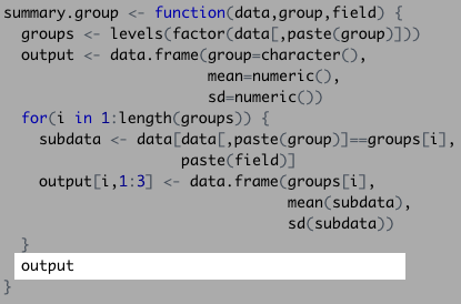
Now this function will run, but there’s still one piece we’re missing. We need to provide a value.
In this function, the value we want is the output object, which is the data frame containing our summary statistics. We can merely add the output reference at the end, outside the control flow:
  summary.group <- function(data,group,field) {
    groups <- levels(factor(data[,paste(group)]))
    output <- data.frame(group=character(),
                         mean=numeric(),
                         sd=numeric())
    for(i in 1:length(groups)) {
      subdata <- data[data[,paste(group)]==groups[i],
                      paste(field)]
      output[i,1:3] <- data.frame(groups[i],
                                  mean(subdata),
                                  sd(subdata))
      }
    output
    }
If we run this function with the Bond data frame, we’ll get this result:
summary.group(bond,"actor","gross")## group mean sd
## 1 Daniel Craig 820.3165 222.57396
## 2 George Lazenby 505.8998 NA
## 3 Pierce Brosnan 510.9380 30.61869
## 4 Roger Moore 550.8332 177.63450
## 5 Sean Connery 724.8824 213.95672
## 6 Timothy Dalton 333.1230 67.833948.9 Breaking Down the Function We Just Made
If you’re new to control flows, this probably confused you.
To make it easier, I’m going to show you step-by-step how this function took the Bond data and created this output.
First, the function reviewed the group we defined and created a vector with the members of that group.
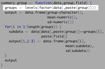
In this instance, that would include the Bond actors:
## [1] "Daniel Craig"   "George Lazenby" "Pierce Brosnan" "Roger Moore"
## [5] "Sean Connery"   "Timothy Dalton"
Second, the function created an empty data frame that will later store the actor names, their mean, and their standard deviation:
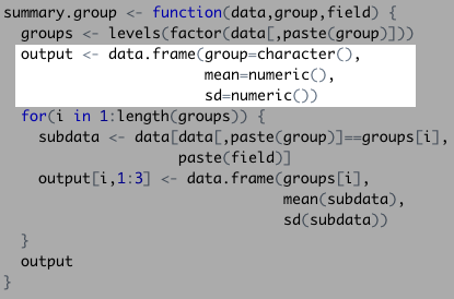
Our function then started a control flow, which will evaluate each actor’s data to fill the data frame we just created:
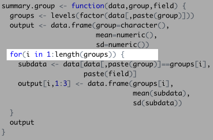
Next, it filtered the Bond data set down to the first actor:
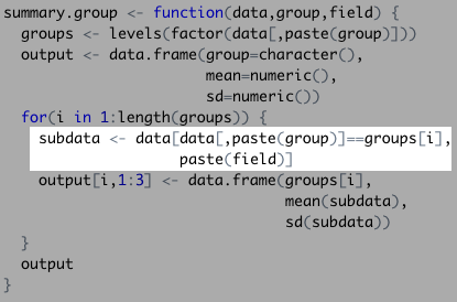
Really, this function filtered the Bond data set in a similar way to the code below:
## [1] 1108.5610 880.6692 669.7895 622.2464The function then took the subdata and calculated our summary statistics. This populated the empty data set one by one…
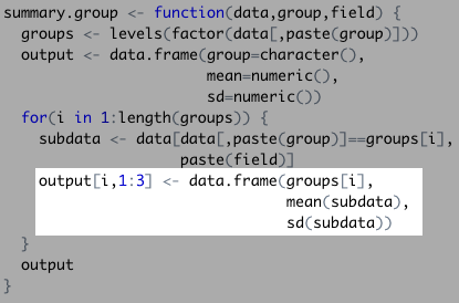
…with each new row looking something like this:
##      groups.1. mean.subdata. sd.subdata.
## 1 Daniel Craig      820.3165     222.574
And finally, it displayed the complete data frame once it finished with the control flow!
8.10 Assigning Functions Outputs a Name
Any objects named within a function are not saved in your R environment. To save the results, you need to assign the executed function a name, like you would with any other object.
  bond_eval <- summary.group(bond,"actor","gross")
  bond_eval
## group mean sd
## 1 Daniel Craig 820.3165 222.57396
## 2 George Lazenby 505.8998 NA
## 3 Pierce Brosnan 510.9380 30.61869
## 4 Roger Moore 550.8332 177.63450
## 5 Sean Connery 724.8824 213.95672
## 6 Timothy Dalton 333.1230 67.83394This can apply to any existing functions.
8.11 Things to Remember
- Functions are the only object type that modifies other objects
- Functions require an argument to execute and typically outputs a value
- Packages store previously built functions that you can utilize
- You can build your own functions to suit your R programming needs
- Control flows or “loops” are a handy way to automate data management tasks at a granular level
8.12 Exercises
Try to see if you can complete the following exercises. Answers are in the back of the book!
- Modify the simple standard deviation function we wrote and change it to calculate mean. Do this without using the built-in
meanfunction. - Alter the
summary.groupfunction to include median, maximum, and minimum values. - Write a function for the Fibonacci Sequence, which ends at a number you choose. You’ll need to use a control flow to accomplish this and a default value for the end of the sequence. (Hint: You won’t use the
for(var in seq) exprcontrol flow. Execute?Controlto use a different version.)